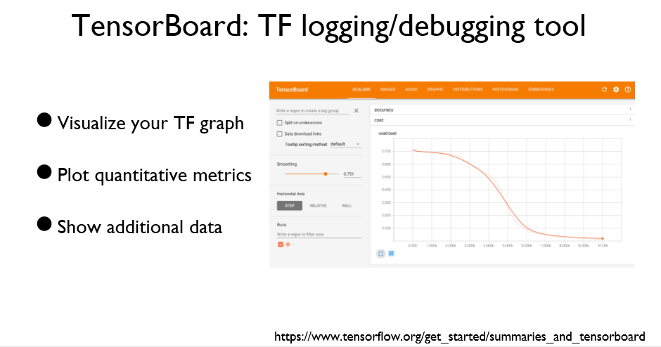
TensorBoard는 Tensorflow 그래프를 시각화 할 수 있는 툴이다.
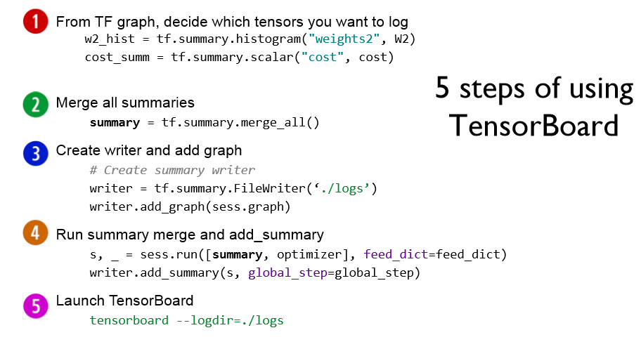
5가지 단계를 추가하면 TensorBoard를 사용할 수 있다.
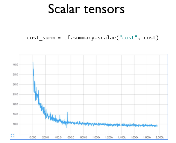
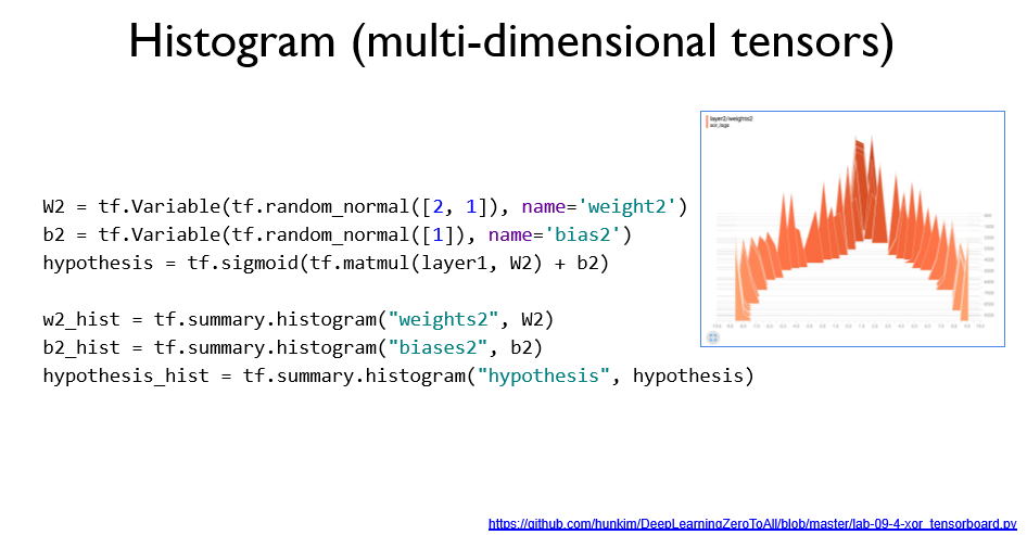
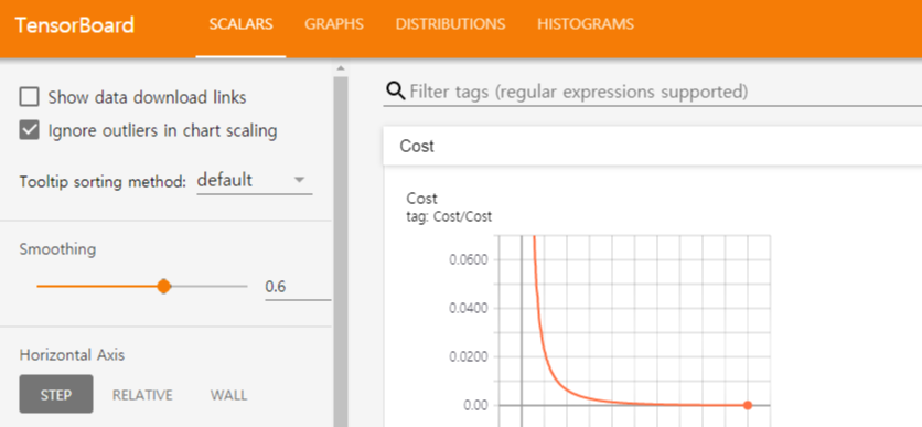
스칼라 값과 히스토그램 값을 시각화 할 수 있다.
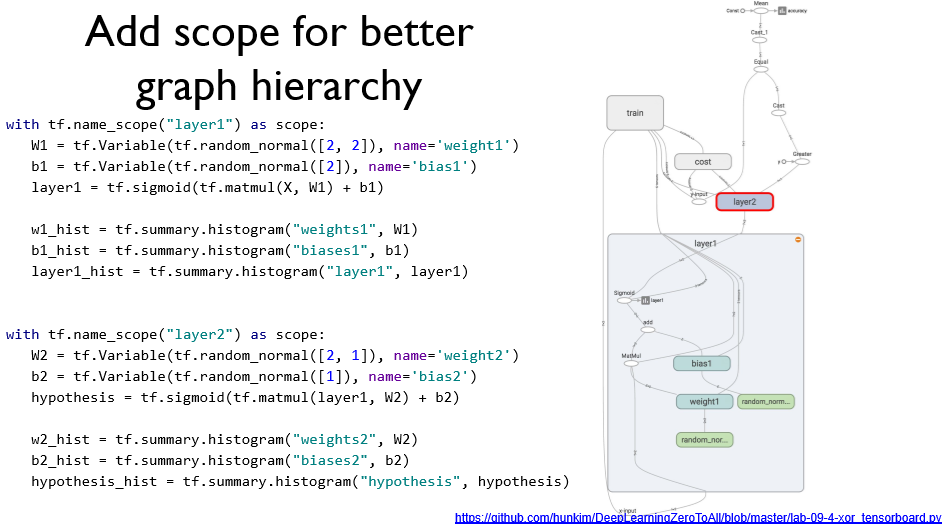
Scope를 이용하면 좀더 깔끔한 Graph 구성이 가능하다. (Like 서랍장)
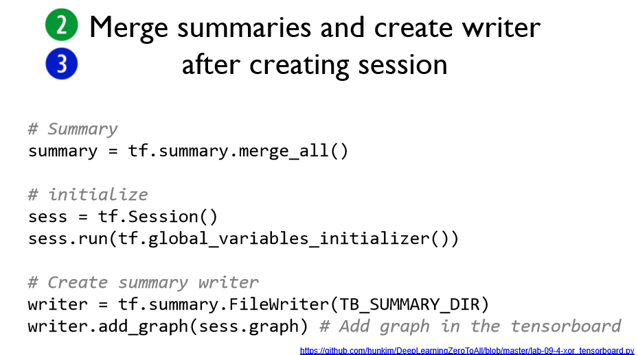
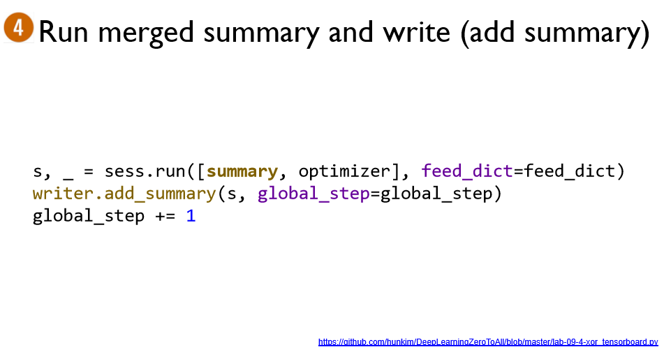
merge_all()를 이용하여 모두 합친 후 세션을 이용하여 Summary를 저장한다.

터미널에 명령어를 입력하여 TensorBoard를 볼 수 있는 주소를 얻을 수 있다.
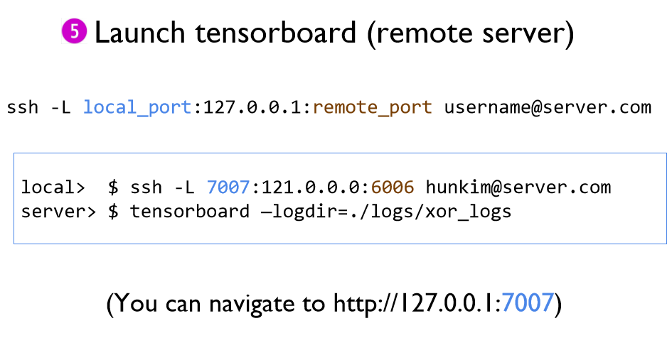
* 원격 서버로 TensorBoard를 사용할 수 있다.
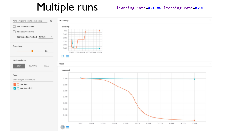
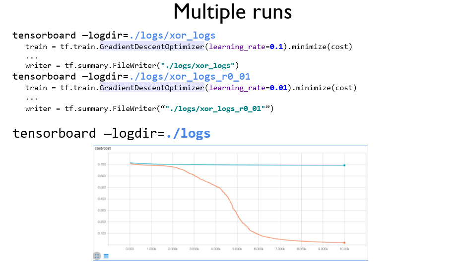
같은 폴더 안에 여러 log들을 저장하면 동시에 비교가 가능하다.
+ 추가
상위 버전에서는 터미널에 입력하는 명령어가 약간 달라졌다.
tensorboard --logdir PATH
* PATH : log 디렉토리 경로
터미널에 위의 명령어를 입력하지 않고 주피터 노트북 환경에서 바로 실행시키는 방법이 있다.
아래 명령어를 이용하여 jupyter-tensorboard를 설치하자.
pip install jupyter-tensorboard
출처: https://lucycle.tistory.com/274 [LuCycle의 잡동사니]
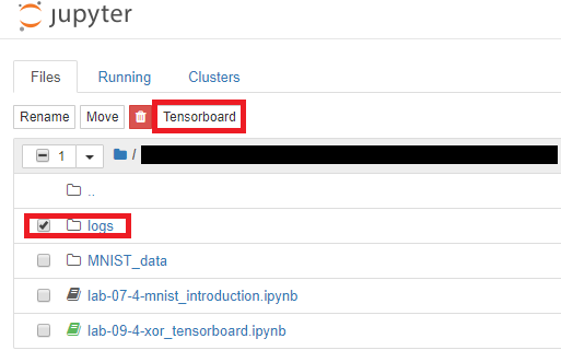
그 다음 log 디렉토리를 체크하면 Tensorboard 표시가 뜨게 된다!
이를 누르면 Tensorboard가 열리게 된다.
코드
|
1
2
3
4
5
6
7
8
9
10
11
12
13
14
15
16
17
18
19
20
21
22
23
24
25
26
27
28
29
30
31
32
33
34
35
36
37
38
39
40
41
42
43
44
45
46
47
48
49
50
51
52
53
54
55
56
57
58
59
60
61
62
63
64
65
66
67
68
69
70
|
# Lab 9 XOR
import tensorflow as tf
import numpy as np
tf.set_random_seed(777) # for reproducibility
x_data = np.array([[0, 0], [0, 1], [1, 0], [1, 1]], dtype=np.float32)
y_data = np.array([[0], [1], [1], [0]], dtype=np.float32)
X = tf.placeholder(tf.float32, [None, 2], name="x")
Y = tf.placeholder(tf.float32, [None, 1], name="y")
with tf.name_scope("Layer1"):
W1 = tf.Variable(tf.random_normal([2, 2]), name="weight_1")
b1 = tf.Variable(tf.random_normal([2]), name="bias_1")
layer1 = tf.sigmoid(tf.matmul(X, W1) + b1)
tf.summary.histogram("W1", W1)
tf.summary.histogram("b1", b1)
tf.summary.histogram("Layer1", layer1)
with tf.name_scope("Layer2"):
W2 = tf.Variable(tf.random_normal([2, 1]), name="weight_2")
b2 = tf.Variable(tf.random_normal([1]), name="bias_2")
hypothesis = tf.sigmoid(tf.matmul(layer1, W2) + b2)
tf.summary.histogram("W2", W2)
tf.summary.histogram("b2", b2)
tf.summary.histogram("Hypothesis", hypothesis)
# cost/loss function
with tf.name_scope("Cost"):
cost = -tf.reduce_mean(Y * tf.log(hypothesis) + (1 - Y) * tf.log(1 - hypothesis))
tf.summary.scalar("Cost", cost)
with tf.name_scope("Train"):
train = tf.train.AdamOptimizer(learning_rate=0.01).minimize(cost)
# Accuracy computation
# True if hypothesis>0.5 else False
predicted = tf.cast(hypothesis > 0.5, dtype=tf.float32)
accuracy = tf.reduce_mean(tf.cast(tf.equal(predicted, Y), dtype=tf.float32))
tf.summary.scalar("accuracy", accuracy)
# Launch graph
with tf.Session() as sess:
# tensorboard --logdir=./logs/xor_logs
merged_summary = tf.summary.merge_all()
writer = tf.summary.FileWriter("./logs/xor_logs_r0_01")
writer.add_graph(sess.graph) # Show the graph
# Initialize TensorFlow variables
sess.run(tf.global_variables_initializer())
for step in range(10001):
_, summary, cost_val = sess.run(
[train, merged_summary, cost], feed_dict={X: x_data, Y: y_data}
)
writer.add_summary(summary, global_step=step)
if step % 100 == 0:
print(step, cost_val)
# Accuracy report
h, p, a = sess.run(
[hypothesis, predicted, accuracy], feed_dict={X: x_data, Y: y_data}
)
print(f"\nHypothesis:\n{h} \nPredicted:\n{p} \nAccuracy:\n{a}")
|
'모두를 위한 딥러닝' 카테고리의 다른 글
| [DL] 모두를 위한 딥러닝 10-2 Initialize weights (0) | 2022.04.05 |
|---|---|
| * [DL] 모두를 위한 딥러닝 10-1 ReLU (0) | 2022.04.05 |
| [DL] 모두를 위한 딥러닝 9-3 Tensorflow를 이용한 XOR구현 (0) | 2022.04.04 |
| * [DL] 모두를 위한 딥러닝 9-2 Backpropagation (0) | 2022.04.03 |
| [DL] 모두를 위한 딥러닝 9-1 Neural Nets(NN) for XOR (0) | 2022.04.03 |